MACCs: Marginal Abatement Cost Curve Reports

Introduction

Marginal Abatement Cost Curves (MACCs) are a useful tool for assessing the cost and abatement potential of various mitigation options and for prioritizing which of a list of potential measures might be most actively pursued.

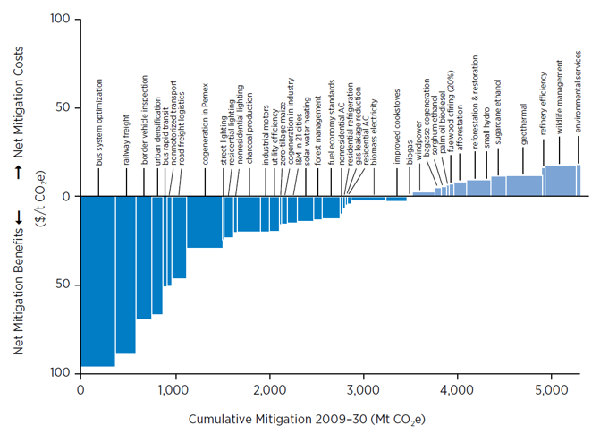
A typical example of a Marginal Abatement Cost Curve (MACC).
Source: Mexico Low Carbon Country Case Study, World Bank ESMAP

MACCs plot cumulative emissions reductions from successive mitigation options (e.g. tonnes of GHGs avoided in CO2e) against the incremental cost per unit of emission reduction (e.g. $/T CO2e). A key property of a MACC is that, for any given set of options the area enclosed by the options equals the cumulative avoided cost of those options. A MACC makes it easy to see which options are low or negative cost (negative cost options appear below the X axis) and which options have the largest mitigation potential (those with the widest bars).

Approaches for Calculating MACCs

As described in Sathaye and Meyers (1995), there are three typical approaches for constructing MACCs:

The Partial Approach: In this method, each option is evaluated separately versus a reference technology. Incremental changes in emissions and costs are calculated and ranked according to their cost effectiveness. Options are ranked independently, ignoring possible interdependence among options. This approach is fast and simple, but theoretically unsatisfactory, and may lead to misinterpretations.
The Retrospective Approach: The first step in this approach is a separate ranking of the technology options: a task identical to that used in the partial approach. Next, the most cost-effective option (lowest $/Ton) is selected and incremental results are calculated relative to a no-policy baseline case. This gives the first block in the cost curve. Next, the second most cost-effective project is included in the model and new calculations are performed. Results are compared to the first option and a new block is established, and so on. This approach requires multiple calculation passes to properly asses how each option may interact with all previously implemented options and thus is considerably slower than the Partial Approach. However, it has the advantage that it more fully takes into account the interdependence among options and previously implemented option. Note however that even the retrospective approach does not consider the interactions between more expensive options on previously chosen (cheaper) options. This may be important, especially in cases where implementation of demand-side options results in significant changes on the supply side. Only a fully integrated analysis can account for these interactions.
The Integrated Systems Approach: This approach requires the existence of a well defined baseline, and an integrated energy system optimization model where the supply side automatically responds to even marginal changes on the demand side in each model run. The idea is to determine any point on the cost curve as the least-cost solution for the total energy system, in which all demand and supply system parameters can vary. This approach aims to take into account all the inter-dependencies within the system, as represented by the energy systems model. A least-cost curve can in principle only be established through use of a cost-minimizing optimization model. A MACC is typically calculated from such models by settings different maximum emission constraints and then examining which set of options the model implements in order to meet those constraints and at what cost. In an optimization approach, the model itself selects the configuration of the energy system that satisfies different emission targets at a minimum cost. The disadvantage of the integrated systems approach is that the inter-dependencies between supply and demand options make it difficult to identify impacts of single options separately, and a strict ranking of options is not possible since the emission reductions achieved as one moves up the cost curve result from the use of several interlinked options. Note that while LEAP does support integrated modeling, it does not currently plot MACC curves based on this approach.

MACCs in LEAP can be used to examine the implementation of a range of different measures, with each measure represented by one of LEAP's scenarios. LEAP MACCs are calculated using either the slower but more thorough Retrospective Approach or the faster but less thorough Partial Approach. Typically, a MACC will show increasing costs from left to right, but due to interactive effects among scenarios this may not always be the case.

Under the Retrospective Approach, LEAP calculates MACCs by performing multiple passes of its standard scenario calculations. Each pass identifies the most cost-effective remaining scenario and then removes that scenario from consideration before recalculating the remaining scenarios. This process continues until only one scenario remains. Note that each scenario implemented will likely affect the costs and abatement potential of subsequently implemented scenarios.

Under the Partial Approach, LEAP calculates all scenarios in a single pass, and simply plots the cost of each scenario relative to the counter factual (baseline) scenario, ignoring potential interactions among those scenarios.

Setting Up MACC Reports

MACC reports are a special type of report displayed in the Summaries view. To create a MACC report, first click on the Manage Summaries screen, and add a new named Marginal Abatement Cost Curve summary report.

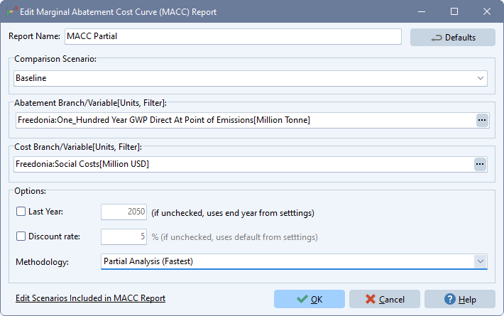LEAP's MACC reports are highly configurable via the MACC Edit () screen shown here. From this screen you can specify the comparison or counter factual scenario (typically a non-policy baseline scenario). You can also select the LEAP variables that will be used to represent overall social costs and impacts. By default, these are total system-wide social costs and total 100-year global warming potential. Use the Branch/Variable selection wizard to specify the branch, variable, units, scaling factor and any special results filters for the abatement and cost variables. Other options let you override the default end year and discount rate parameters in the MACC calculations. By default these are the values specified in the General: Settings screen. Currently, all MACC reports show cumulative costs and abatement potential. Use the Calculation Passes option to specify if the MACC is calculated using the more thorough (but slower) Retrospective Approach or the faster (but less thorough) Partial Approach.

You can create multiple MACC reports, each with different names and different settings. For example, one report might show avoided GHGs, a second might show avoided particulate emissions, and a third might show avoided health impacts (for example when using LEAP with IBC). Use the Add button () in the Manage Summaries screen to create additional MACC reports.

The scenarios included in a MACC report will be those selected for use in MACCs via the General: Manage Scenarios screen. Check the Include in MACC Report option for each scenario you want plotted in your MACC report. Note that, because LEAP's MACC calculations automatically find scenarios in order from the most to least cost-effective, it is important that the scenarios you select are not themselves packages of other scenarios already included for display in the MACC report. For example, don't include an overall mitigation scenario as well as individual scenarios that from which the mitigation scenario inherits. If you do include scenarios twice (alone and as part of a package), when you go to display a MACC, an error message will appear and the calculations will be halted.

Displaying MACC Reports

Once a MACC curve has been set up, return to the Summaries screen and select it. MACC reports are created by iteratively searching for the most cost-effective scenarios in such a way that each scenario implemented will likely affect the costs and abatement potential of subsequently implemented scenarios. For this reason, calculating a MACC report requires multiple passes of LEAP's standard calculations. For this reason, and unlike with other types of results in LEAP, MACC results must be manually refreshed any time a LEAP data set is changed. Use the Refresh MACC () button to recalculate a MACC report.

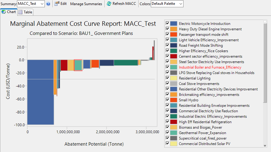
MACCs can be displayed ether in table or chart format. MACC tables show each scenario calculated as rows and the abatement potential, cost and unit cost for each scenario as columns. A sample MACC chart is shown below. This follows the standard format for MACC charts, with abatement potential displayed on the X axis and the marginal cost per unit of abatement of each option (after the previous options were also implemented) displayed on the Y axis. Each option is shown as a variable width colored bar. The average unit abatement cost is also displayed as a line on the bar.

Various on-screen options displayed in a tool bar on the right of the screen can be used to customize the display of the MACC chart. You can increase () or decrease () the number of decimals displayed in the table, change the display of grid lines on the chart (), change the table font (), export tables to Excel (), print and preview tables and charts (), copy charts and tables to the Windows clipboard (), and export charts to PowerPoint ().